Chapter 6
Taking All Kinds of Samples
IN THIS CHAPTER
 Grasping the concept of statistical error
Setting up your sampling frame
Executing a sampling strategy
Sampling — or taking a sample — is an important concept in statistics. As described in Chapter 3, the purpose of taking a sample — or a group of individuals from a population — and measuring just the sample is so that you do not have to conduct a census and measure the whole population. Instead, you can measure just the sample and use statistical approaches to make inferences about the whole, which is called inferential statistics. You can estimate a measurement of the entire population, which is called a parameter, by calculating a statistic from your sample.
Some samples do a better job than others at representing the population from which they are drawn. We begin this chapter by digging more deeply into some important concepts related to sampling. We then describe specific sampling approaches and discuss their pros and cons.
Making Forgivable (and Non-Forgivable) Errors
A central concept in statistics is that of error. In statistics, the term error sometimes means what you think it means — that a mistake has been made. In those cases, the statistician should take steps to avoid the error. But other times in statistics, the term error refers to a phenomenon that is unavoidable, and as statisticians, we just have to cope with it.
For example, imagine that you had a list of all the patients of a particular clinic and their current ages. Suppose that you calculated the average age of the patients on your list, and your answer was 43.7 years. That would be a population parameter. Now, let’s say you took a random sample of 20 patients from that list and calculated the mean age of the sample, which would be a sample statistic. Do you think you would get exactly 43.7 years? Although it is certainly possible, in all likelihood, the mean of your sample — the statistic — would be a different number than the mean of your population — the parameter. The fact that most of the time a sample statistic is not equal to the population parameter is called sampling error. Sampling error is unavoidable, and as statisticians, we are forced to accept it.
Now, to describe the other type of error, let’s add some drama. Suppose that when you went to take a sample of those 20 patients, you spilled coffee on the list so you could not read some of the names. The names blotted out by the coffee were therefore ineligible to be selected for your sample. This is unfair to the names under the coffee stain — they have a zero probability of being selected for your sample, even though they are part of the population from which you are sampling. This is called undercoverage, and is considered a type of non-sampling error. Non-sampling error is essentially a mistake. It is where something goes wrong during sampling that you should try to avoid. And unlike sampling error, undercoverage is definitely a mistake you should avoid making if you can (like spilling coffee).
Framing Your Sample
In the previous example, the patient list is considered your sampling frame. A sampling frame represents the practical representation of the population from which you are literally drawing your sample. We described this list as a printout of patient names and their ages. Suppose that after the list was printed, a few more patients joined the clinic, and a few patients stopped using the clinic because they moved away. This situation means that your sampling frame — your list — is not a perfect representation of the actual population from which you are drawing your sample.
 If you omit population members from your sampling frame, you get undercoverage, which is a form of non-sampling error (the type of error you want to avoid). Also, if you accidentally include members in your sampling frame who are not part of the population (such as patients who moved away from the clinic after you printed your list), and they actually get sampled, you have another form of non-sampling error. Non-sampling error can also creep in from making sloppy measurements during data collection, or making poor choices when designing your study. Chapter 8 provides guidance on how to minimize errors during data collection, and Chapters 5 and 7 provide advice on study design.
Another sampling-related vocabulary word is simulation. When talking about sampling, a simulation refers to pretending to have data from an entire population from which you can take samples, and then taking different samples to see what happens when you analyze the data. That way, you can make sample statistics while peeking at what the population parameters actually are behind the scenes to see how they behave together.
One simulation you could do to illustrate sampling error in Microsoft Excel is to create a column of 100 values that represent ages of imaginary patients at a clinic as an entire population.
- If you calculated the mean of these 100 values, you would be doing a simulation of the population parameter.
- If you randomly sampled 20 of these values and calculated the mean, you would be doing a simulation of a sample statistic.
- If you compared your parameter to the statistic to see how close they were to each other, you would be doing a simulation of sampling error.
So far we’ve reviewed several concepts related to the act of sampling. However, we haven’t yet examined different sampling strategies. It matters how you go about taking a sample from a population; some approaches provide a sample that is more representative of the population than other approaches. In the next section, we consider and compare several different sampling strategies.
Sampling for Success
As mentioned earlier, the purpose of taking measurements from a sample of a population is so that you can use it to perform inferential statistics, which enables you to make estimates about the population without having to measure the entire population. Theoretically, you want the statistics from your sample to be as close as possible to the population parameters you are trying to estimate. To increase the likelihood that this happens, you should try your best to draw a sample that is representative of the population.
You may be wondering, “What is the best way to draw a sample that is representative of the background population?” The honest answer is, “It depends on your resources.” If you are a government agency, you can invest a lot of resources in conducting representative sampling from a population for your studies. But if you are a graduate student working on a dissertation, then based on resources available, you probably have to settle for a sample that is not as representative of the population as a government agency could afford. Nevertheless, you can still use your judgment to make the wisest decisions possible about your sampling approach.
Taking a simple random sample
Taking a simple random sample (SRS) is considered a representative approach to sampling from a background population. In an SRS, every member of the population has an equal chance of being selected randomly and included in the sample. As an example, recall the printout of the current patient list from a clinic discussed in the previous section. Considering that list a clinical population, imagine that you used scissors to cut the list up so that each name was on its own slip of paper, and then you put all the slips of paper into a hat. If you want to take an SRS of 20 patients, you could randomly remove 20 names from the hat. The SRS would be seen as a highly representative sample.
 In practice, an SRS is usually taken using a computer so that you can take advantage of a random number generator (RNG) (and do not have to cut up all that paper). Imagine that the patient list from which you were sampling was not printed on paper, but was instead stored in a column in a spreadsheet in Microsoft Excel. You could use the following steps to take an SRS of 20 patients from this list using the computer:
Create a column containing random numbers.
You could create another column in the spreadsheet called “Random” and enter the following formula into the top cell in the column: =RAND(). If you drag that cell down so that the entire column contains this command, you will see that Excel populates each cell with a random number between 0 and 1. Each time Excel evaluates, the random number gets recalculated.
- Sort the list by the random number column.
- Select the top 20 rows from the list.
This process ensures that your sample of 20 patients was taken completely at random. Statistical packages like those described in Chapter 4 have RNG commands similar to the one in Excel.
 Learners sometimes think that as long as they sort a spreadsheet of data by a column containing any value and then select a sample of rows from the top, that they have automatically obtained an SRS. This is not correct! If you think about it more carefully, you will realize why. If you sort names alphabetically, you will see patterns in names (such as religious names, or names associated with certain languages, countries, or ethnicities). If you sort by another identifying column, such as email address or city of residence, you will again see patterns in the data. If you attempt to take an SRS from such data, it will be biased, not random, and not be representative. That is why it is important to use a column with an RNG in it for sorting if you are taking an SRS electronically.
Taking an SRS intuitively seems like the optimal way to draw a representative sample. However, there are caveats. In the previous example, you started with a clinical population in the form of a printed or electronic list of patients from which you could draw a sample. But what if you want to sample from patients presenting to the emergency department during a particular period of time in the future? Such a list does not exist. In a situation like that, you could use systematic sampling, which is explained later in the section “Engaging in systematic sampling.”
Another caveat of SRS is that it can miss important subgroups. Imagine that in your list of clinic patients, only 10 percent were pediatric patients (defined as patients under the age of 18 years). Because 10 percent of 20 is two, you may expect that a random sample of 20 patients from a population where 10 percent are pediatric would include two pediatric patients. But in practice, in a situation like this, it would not be unusual for an SRS of 20 patients to include zero pediatric patients. If your SRS needs to ensure representation by certain subgroups, then you should consider using stratified sampling instead.
Taking a stratified sample
In the previous section, we discussed a scenario where 10 percent of the patients of a clinic are pediatric patients, and taking a sample of 20 using an SRS from a list of the clinic population runs the risk of not including any pediatric patients. If pediatric patients were important to the study, then this problem can be solved with stratified sampling. The word stratum refers to a layer (as you see in a layer cake), and the word strata is the plural of stratum. Stratified sampling can be seen as sampling from strata, or layers.
In our scenario, if you choose to draw a stratified sample by age groups, you would first have to separate the list into a pediatric list and a list of everyone else. Then, you could take an SRS from each. Because you are concerned about each stratum, you could make a rule that even though pediatric patients make up only 10 percent of the background population, you want them to make up 50 percent of your sample. If you did that, then when you took your SRS, you would oversample from the pediatric list and select 10, while also taking an SRS of 10 from the list of everyone else.
Drawing a stratified sample requires you to weight your overall estimate, or else it will be biased. As an example, imagine that 15 percent of pediatric patients had an oral health condition, and 50 percent of the rest of the patients had an oral health condition. In a stratified sample of 20 patients where you draw 10 from the pediatric population and 10 from the rest of the population, because the pediatric population is oversampled (because they only make up 10 percent of the background population but make up 50 percent of our sample), if weights are not applied, the estimate of the percentage of the population with an oral health condition would be artificially reduced. That is why it is necessary to apply weights to overall estimates derived from a stratified sample.
If you are familiar with large epidemiologic surveillance studies such as the National Health and Nutrition Examination Survey (NHANES) in the United States, you may be aware that extremely complex stratified sampling is used in the design and execution of such studies. Stratified sampling in these studies is unlike the simple example described earlier, where the stratification involves only two age groups. In surveillance studies like NHANES, there may be stratified sampling based on many characteristics, including age, gender, and location of residence. If you need to select factors on which to stratify, trying looking at what factors were used for stratification in historical studies of the same population. The kind of stratified sampling used in large-scale surveillance studies is reviewed later in this chapter in the section “Sampling in multiple stages.”
Engaging in systematic sampling
Earlier you considered a scenario where a clinic had a printed list of the entire population of patients from which an SRS could be drawn. But what if you want to sample from the population of patients who present to a particular emergency department tonight between 6 p.m. and midnight? There is no convenient list from which to draw such a sample. In a scenario like this, even though you can’t draw an SRS, you want to use a system for obtaining a sample such that it would be representative of the underlying population. To do that, you could use systematic sampling.
Imagine you are surveying a sample of patients about their opinions of waiting times at a particular emergency department, and you are doing this in the time window of between 6 p.m. and midnight tonight. To take a systematic sample of this population, follow these steps:
Select a small number.
This is your starting number. If you select three, this means that — starting at 6 p.m. — the first patient to whom you would offer your survey would be the third one presenting to the emergency department.
Select another small number.
This is your sampling number. If you select five, then after the first patient to whom you offered the survey, you would ask every fifth patient presenting to the emergency department to complete your survey.
Continue sampling until you have the size sample you need (or the time window expires).
Chapter 4 describes the software G*Power that can be used for making sample-size calculations.
In systematic sampling, you are technically starting at a random individual, then selecting every kth member of the population, where k stands for the sampling number you selected.
Systematic sampling is not representative if there are any time-related cyclic patterns that could confer periodicity onto the underlying data. For example, suppose that it was known that most pediatric patients present to the emergency department between 6 p.m. and 8 p.m. If you chose to collect data during this time window, even if you used systematic sampling, you would undoubtedly oversample pediatric patients.
Sampling clusters
Another challenge you may face as a biostatistician when it comes to sampling from populations occurs when you are studying an environmental exposure. The term exposure is from epidemiology and refers to a factor hypothesized to have a causal impact on an outcome (typically a health condition). Examples of environmental exposures that are commonly studied include air pollution emitted from factories, high levels of contaminants in an urban water system, and environmental pollution and other dangers resulting from a particular event (such as a natural disaster).
Consider the scenario where parents in a community are complaining that a local factory is emitting pollutants that they believe is resulting in a higher rate of leukemia being diagnosed in the community’s youth. To study whether the parents are correct or not, you need to sample members of the population based on their proximity to the factory. This is where cluster sampling comes in.
Planning to do cluster sampling geographically starts with getting an accurate map of the area from which you are sampling. In the United States, each state is divided up into counties, and each county is further subdivided into smaller regions determined by the U.S. census. Other countries have similar ways their maps can be divided along official geographic boundaries. In the scenario described where a factory is thought to be polluting, the factory could be placed on the map and lines drawn around the locations from which a sample should be drawn. Different methodologies are used depending upon the specific study, but they usually involve taking an SRS of regions and from the sampled regions known as clusters, taking an SRS of community members for study participation.
But cluster sampling is not only done geographically. As another example, clusters of schools may be selected based on school district, rather than geography, and an SRS drawn from each school. The important takeaway from cluster sampling is that it is a sampling strategy optimized for drawing a representative sample when studying an exposure known to be uneven across the population.
Sampling at your convenience
If you have read this chapter from the beginning until now, you may be feeling a little exasperated. And that may be because all the sampling strategies we have discussed so far — SRS, stratified sampling, systematic sampling, and cluster sampling — involve a lot of work for the researcher. In an SRS, you need to have a list of the population from which to draw, and in stratified sampling, you have to know the value of the characteristics on which you want to stratify your sample. Each of these features makes designing your sampling frame more complicated.
Thinking this way, both systematic sampling and cluster sampling also add complexity to your sampling frame. In systematic sampling, whether you use a static list or you sample in real time, you need to keep track of the details of your sampling process. In cluster sampling, you may be using a map or system of groupings from which to sample, and that also involves a lot of recordkeeping. You may be asking by now, “Isn’t there an easier way?”
Yes! There is an easier and more convenient way: convenience sampling. Convenience sampling is what you probably think it is — taking a sample from a population based on convenience. For example, when statistics professors want to know what students think about a new policy on campus, they can just ask whoever is in their classes, as those students are a convenient sample of the student population.
The problem is that the answer they get may be very biased. Most of the students in their classes may come from the sciences, and those studying art or literature may feel very differently about the same policy. Although our convenience sample would be a valid sample of the background population of students, it would be such a biased sample that the results would probably be rejected by the rest of the faculty — especially those from the art and literature departments!
 Given that the results from convenience samples are usually biased, you may think that convenience sampling is not a good strategy. In actuality, convenience sampling comes in handy if you have a relatively low-stakes research question. Customer satisfaction surveys are usually done with convenience samples, such as those placing an order on a restaurant’s app. It is simple to program such a survey into an app, and if the food quality is terrific and the service terrible, it will be immediately evident even from a small convenience sample of app users completing the survey.
While low-stakes situations are fine for convenience sampling, high-stakes situations — like studying whether a new drug is safe and/or effective — require study designs and sampling approaches completely focused on minimizing bias. As with SRS, convenience sampling is prone to omitting important subgroups from the sample. Minimizing bias through sampling and other strategies is covered in detail in Chapter 5, which examines clinical research and describes how researchers must present a well-defined protocol that includes selection criteria, a sampling plan, and an analytic plan that undergoes regulatory approval prior to the commencement of research activities. Other strategies for minimizing bias are presented in Chapters 7 and 20, which cover study designs and causal inference.
Sampling in multiple stages
When conducting large, epidemiologic surveillance studies, it is necessary to do an especially good job of sampling, because governments use results from these studies on which to base public policy. As an example, because being obese puts community members at risk for serious health conditions, government public health agencies have a vested interest in making accurate estimates of the rates of obesity in their communities.
For this reason, to strive to obtain a representative sample, researchers designing large epidemiologic surveillance studies use multi-stage sampling. Multi-stage sampling is a general term for using multiple sampling approaches at different stages as part of a strategy to obtain a representative sample. Figure 6-1 provides a schematic describing the multi-stage sampling in the U.S. surveillance study mentioned earlier, NHANES.
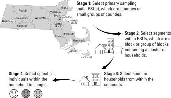
© John Wiley & Sons, Inc.
FIGURE 6-1: Example of multi-stage sampling from the National Health and Nutrition. Examination Survey (NHANES).
As shown in Figure 6-1, in NHANES, there are four stages of sampling. In the first stage, primary sampling units, or PSUs, are randomly selected. The PSUs are made up of counties, or small groups of counties together. Next, in the second stage, segments — which are a block or group of blocks containing a cluster of households — are randomly selected from the counties sampled in the first stage. Next, in the third stage, households are randomly selected from segments. Finally, in stage four, to select each actual community member who will be offered participation in NHANES, an individual is randomly selected from each household sampled in the third stage.
That is how a sample of 8,704 individuals participating in NHANES in 2017–2018 was selected to represent the population of the approximately 325 million people living in the United States at that time. The good news is that biostatisticians work on teams to develop a multi-stage sampling strategy — no one is expected to set up something so complicated all by themselves.